Improving Direct Lighting Material Occlusion - Part 2
 |
|---|
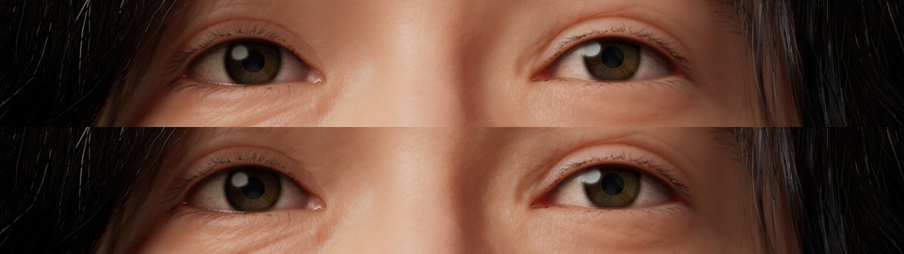
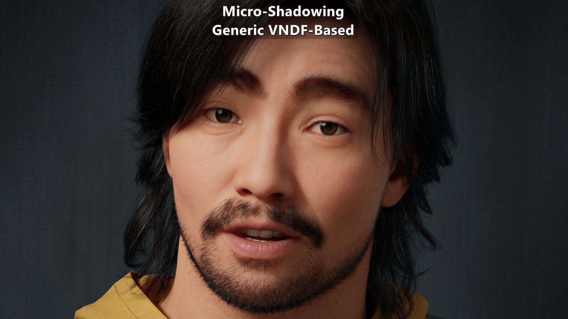
| Skin with micro-occlusion at the top, and micro-shadowing below. Both are using the same micro-occlusion data and were taken with the exact same exposure. |
Last time I went over micro-occlusion, existing micro-shadowing approaches, and provided an analytical alternative approach. But at the end of that post I went over the fact that none of the results of those approaches depended on the definition of the microsurface.
The microsurface is not only relevant to the specular component, but it is also becoming relevant to the diffuse component. While some engines still rely on a Lambert diffuse bidirectional reflectance distribution function (BRDF), many transitioned to diffuse BRDFs that have other characteristics such as being roughness-aware. Some diffuse BRDFs like Oren-Nayar’s need a custom roughness parameter, but other ones leverage a shared definition of a microsurface for the specular and diffuse component. That allows them to converge to the same diffuse and specular roughness parameter as they have the same underlaying microsurface.
This time I will be going over a micro-shadowing approach based on a microsurface. This post assumes that you read and understood the content of the previous post in the series.
Framework
Before getting into this specific alternative approach for micro-shadowing, it is important to understand the framework for it. The framework is essentially built on top of microfacet theory, and in particular Eric Heitz, 2014 “Understanding the Masking-Shadowing Function in Microfacet-Based BRDFs”. The relevant components of the framework are:
- Geometric surface. This defines the surface at a mesoscopic and macroscopic scale, and it where the microsurface is on. This is often the combination of the mesh geometry and normal map.
- Rough microsurface. This is the actual surface the light interacts with. The assumption going forward is that the microsurface is composed of microfacets. This is often controlled via a roughness map.
- \({Visibility}\) term. This defines a cone aperture at the scale of the geometric surface that determines the directions that can interact with the microsurface. At \({Visibility=1.0}\) all directions over the hemisphere are visible, and at \({Visibility=0.0}\) all directions over the hemisphere are occluded. This is controlled via a micro-occlusion map. The assumption going forward is that the \({Visibility}\) is expressed in terms of the projected solid angle meaning \({cos\,\theta = \sqrt{1-Visibility}}\).
The implication of this setup is that, unlike previously mentioned micro-shadowing solutions, the micro-shadowing will be done at the microsurface level rather that at the geometric surface level giving more variation to the results.
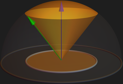
Another relevant aspect is that the intuition coming from the Nusselt analog can be used to relate the \({Visibility}\) term to directions such as incident or outgoing direction.
 |
|---|
| Visibility cone within the unit hemisphere, and visibility disk within the unit disk. \(\theta\) is the angle between the green vector and the blue vector (which corresponds to the geometric surface normal \({\omega_{g}}\)). |
Notation
Because this post is focused on micro-shadowing at the microfacet level, the notation used resembles the notation used on reference papers.
| \({\omega_{g}=(0,0,1)}\) or \(N\) | Geometric surface normal. |
| \({\omega_{o}}\) or \(L\) | Outgoing direction. |
| \({\omega_{i}}\) or \(V\) | Incident direction. |
| \({\omega_{m}}\) | Visible microfacet normal obtained via VNDF sampling. |
| \({Visibility}\) | Visibility cone aperture. |
| \({cos\,\theta=\sqrt{1-Visibility}}\) | Visibility cone angle. |
| \({GenericM_{m}(cos\,\theta,\omega_{m},\omega_{g},\omega_{o},\omega_{i})}\) | Generic micro-shadowing function for a microfacet. |
| \({GenericM_{g}(cos\,\theta,\alpha,\omega_{g},\omega_{o},\omega_{i})}\) | Generic micro-shadowing function for the geometric surface. |
| \({G_{1}(\omega_{i},\omega_{m})}\) | Masking function. |
| \({G_{2}(\omega_{i},\omega_{o},\omega_{m})}\) | Masking-shadowing function. |
| \({D(\omega_{m})}\) | Distribution of normals (NDF). |
| \({D_{\omega_{i}}(\omega_{m})}\) | Distribution of visible normals (VNDF). |
| \({\chi^{+}(a)}\) | Heaviside function: \(1\) when \({a\gt 0}\), and \(0\) when \({a\le 0}\). |
| \({\left\langle \omega_{1}\cdot \omega_{2} \right\rangle}\) | Clamped dot product to the \({[0,1]}\) range. |
| \({u_{1}}\) and \({u_{2}}\) | Uniform random numbers in the \({[0,1)}\) range. |
Generic VNDF-Based Micro-Shadowing
Physically based microsurface models have a statistical description that’s modeled by a microfacet normal distribution function (NDF) and a microsurface profile which models how the microfacets are organized within the microsurface. For a given a microsurface profile, an arbitrary microfacet normal from the NDF may not be visible. That’s why the intention is to sample the distribution of visible normals (VNDF). A single VNDF sample represents a microfacet normal that we can use for micro-shadowing, so now let’s look at the reference function:
\[{\chi^{+}({\left\langle \omega_{g}\cdot \omega_{o} \right\rangle}-cos\,\theta)}\]That’s defined in terms of the geometric surface normal \(\omega_{g}\) which is fine for a perfectly smooth microsurface where all microfacet normals match the geometric normal, but it is problematic as soon as any amount of roughness is introduced. Instead of working with geometric surface normal \(\omega_{g}\), this approach relies on visible microfacet normal \(\omega_{m}\). For this approach the questions that need to be answered to know if a microfacet isn’t micro-shadowed are:
- Is the microfacet facing in a direction within the visibility cone?
- Is the microfacet facing the light within the visibility cone?
To answer them we can use the Nusselt analog. The Nusselt analog provides an easy way to understand the reasoning behind \({cos\,\theta=\sqrt{1-Visibility}}\), and how it can be used to compare the visibility cone to directions. And if we wanted to work in terms of aperture values, its inverse, \({1.0-{(cos\,\theta)}^{2}}\), can be used to know the aperture of the cone created by a direction and the geometric surface normal. While either approach is fine in terms of correctness, the recommendation is to use \({cos\,\theta}\) instead of \({Visibility}\) since \({cos\,\theta}\) is shared across all lights while the directions are unique per light. Based on that, expressions can be created to answer each question:
- “Is the microfacet facing in a direction within the visibility cone?”
- \({\chi^{+}({\left\langle \omega_{g}\cdot \omega_{m} \right\rangle}-cos\,\theta)}\)
- “Is the microfacet facing the light within the visibility cone?”
- \({\chi^{+}({\left\langle \omega_{m}\cdot \omega_{o} \right\rangle}-cos\,\theta)}\)
Since those are the requirements to determine if a microfacet isn’t micro-shadowed, we can put them together:
\[{{\chi^{+}({\left\langle \omega_{g}\cdot \omega_{m} \right\rangle}-cos\,\theta)}{\chi^{+}({\left\langle \omega_{m}\cdot \omega_{o} \right\rangle}-cos\,\theta)}}\]While the expression doesn’t explicitly contain \({\omega_{i}}\), that’s fine as \({\omega_{m}}\) comes from VNDF sampling which depends on \({\omega_{i}}\). And since BRDFs follow Helmholtz reciprocity, we can swap \({\omega_{i}}\) and \({\omega_{o}}\) when desired. But while \({\omega_{m}}\) comes from VNDF sampling, the relevance of that microfacet isn’t solely defined by the VNDF. Let’s look at the definition of the VNDF:
\[{D_{\omega_{i}}(\omega_{m})=\frac{G_{1}(\omega_{i},\omega_{m}){\left\langle \omega_{i}\cdot\omega_{m} \right\rangle}D(\omega_{m})}{\left|\omega_{i}\cdot\omega_{g}\right|}}\]Given its definition, the VNDF doesn’t account for the visible microfacet shadowing. “Microfacet shadowing” is not the same as “micro-shadowing”. Microfacet shadowing deals with the fact that a ray in a \({\omega}\) direction can be intersected by the microsurface itself after the first bounce. Our micro-shadowing function for a visible microfacet needs to account for that, so we want to weight it based on the probability that the microfacet is not shadowed given that it is not masked. \(G_{2}(\omega_{i},\omega_{o},\omega_{m})\) models the masking-shadowing, and \(G_{1}(\omega_{i},\omega_{m})\) models just masking, so we want to weight it by \({\large\frac{G_{2}(\omega_{i},\omega_{o},\omega_{m})}{G_{1}(\omega_{i},\omega_{m})}}\). The resulting function is:
\[{{GenericM_{m}(cos\,\theta,\omega_{m},\omega_{g},\omega_{o},\omega_{i})}={\chi^{+}({\left\langle \omega_{g}\cdot \omega_{m} \right\rangle}-cos\,\theta)}{\chi^{+}({\left\langle \omega_{m}\cdot \omega_{o} \right\rangle}-cos\,\theta)}{\frac{G_{2}(\omega_{i},\omega_{o},\omega_{m})}{G_{1}(\omega_{i},\omega_{m})}}}\]It is important to be aware that the definition of \({\large\frac{G_{2}(\omega_{i},\omega_{o},\omega_{m})}{G_{1}(\omega_{i},\omega_{m})}}\) depends of the microsurface profile and its form for \(G_{2}(\omega_{i},\omega_{o},\omega_{m})\). Assuming the Smith profile, then:
| \({\large \frac{G_{2}(\omega_{i},\omega_{o},\omega_{m})}{G_{1}(\omega_{i},\omega_{m})}=\normalsize G_{1}(\omega_{o},\omega_{m})}\) | Uncorrelated form. |
| \({\large \frac{G_{2}(\omega_{i},\omega_{o},\omega_{m})}{G_{1}(\omega_{i},\omega_{m})}=\frac{G_{1}(\omega_{o},\omega_{m})}{G_{1}(\omega_{o},\omega_{m})+G_{1}(\omega_{i},\omega_{m})-G_{1}(\omega_{o},\omega_{m})G_{1}(\omega_{i},\omega_{m})}}\) | Height-correlated form. |
One last issue is that as \({\left\langle \omega_{g}\cdot \omega_{o} \right\rangle}\) decreases, so do the odds of a microfacet not facing the light within the visibility cone even for \({Visibility=1.0}\). To account for that, micro-shadowing will be expressed in terms of microfacets not micro-shadowed by the hemisphere.
Now we have a setup to micro-shadow a microfacet that we can apply to a given microsurface model. The most commonly used microsurface is Smith + Trowbridge–Reitz (GGX) so that’s the assumption for the rest of the post. With that said, other models such as Beckmann-Spizzichino + V-cavity should work, which is why no attempt is made to find a closed-form solution to the assumed microsurface. Given the Smith + Trowbridge–Reitz (GGX) assumption, the missing component is the VNDF sampling function to obtain \({\omega_{m}}\) for given random uniform numbers \({u_{1}}\) and \({u_{2}}\), direction \({\omega_{i}}\), and GGX \(\alpha\). I decided to go with Jonathan Dupuy and Anis Benyoub, 2023 “Sampling Visible GGX Normals with Spherical Caps”.
Under the Smith profile assumption there is one important aspect to cover for the implementation, and that’s the handling of anisotropy. Distributions such as anisotropic GGX and anisotropic Beckmann use roughness value \(\alpha\) which doesn’t have a single dimension. That impacts the definition of the Smith \(\Lambda\) function which is part of \({G_{1}(\omega)}\). Fortunately, isotropic shape-invariant distributions such as GGX and Beckmann can be transformed into an anisotropic configuration by stretching the surface and vice versa. This means that we can project anisotropic roughness onto a given direction to determine the visible microfacet shadowing.
With those aspects covered, let’s look at the implementation of the generic micro-shadowing function for a Smith + anisotropic Trowbridge–Reitz (GGX) microfacet.
 1void MicroShadowingTermPZGenericVNDFBased(in float cosTheta, in float2 ggxAlpha, in float3 N, in float3 L, in float3 V, in float2 u1u2,
 2	out float outConeResult, out float outHemisphereResult, out float outSampleWeight)
 3{
 4	const float3 M = ImportanceSampleGGXVNDF(V, ggxAlpha, u1u2); // wm
 5	const float projectedGgxAlphaV = ProjectRoughnessGGX(V, ggxAlpha); // Project GGX roughness onto wi
 6	const float projectedGgxAlphaL = ProjectRoughnessGGX(L, ggxAlpha); // Project GGX roughness onto wo
 7
 8	const float NdotM = saturate(dot(N, M));
 9	const float MdotL = saturate(dot(M, L));
10
11	outSampleWeight = ImportanceSampleGGXVNDF_Weight(V, L, M, projectedGgxAlphaL, projectedGgxAlphaV); // G2(wi,wo,wm)/G1(wi,wm)
12	outHemisphereResult = HeavisideFunction(NdotM) * HeavisideFunction(MdotL) * outSampleWeight;
13	outConeResult = HeavisideFunction(NdotM - cosTheta) * HeavisideFunction(MdotL - cosTheta) * outSampleWeight;
14}
Generic Micro-Shadowing of The Surface
Now that we can micro-shadow a microfacet, it is time to micro-shadow the geometric surface by micro-shadowing the microfacets with it. This means that we’ll need to do the numerical integration of:
\[{{GenericM_{g}(cos\,\theta,\alpha,\omega_{g},\omega_{o},\omega_{i})}=\frac{\int_{\Omega} {GenericM_{m}(cos\,\theta,\omega_{m},\omega_{g},\omega_{o},\omega_{i})} \,d\mspace{2mu}{\omega_{m}}}{\int_{\Omega} {GenericM_{m}(0,\omega_{m},\omega_{g},\omega_{o},\omega_{i})} \,d\mspace{2mu}{\omega_{m}}}}\]With that in place \(n\) number of samples can be taken and the feature can be implemented and verified in engine.
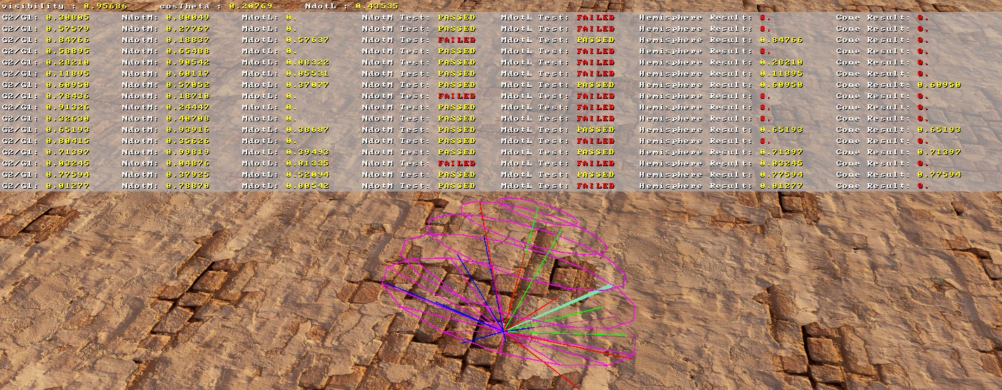 |
|---|
| Debug view of the micro-shadowing by a directional light of a single pixel implemented on Unreal Engine 5. 16 VNDF samples, sun direction in emerald, visibility cone in magenta. Microfacets micro-shadowed by the hemisphere in blue, and by the visibility cone in red. |
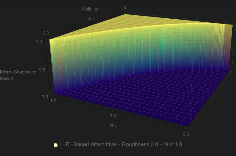
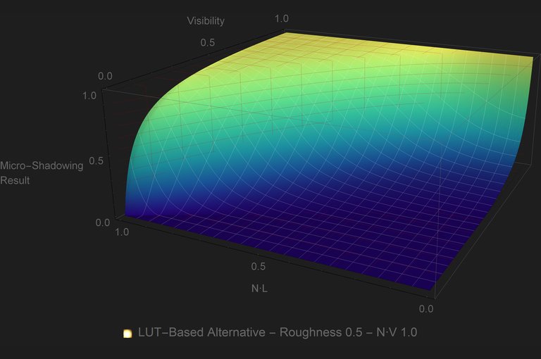
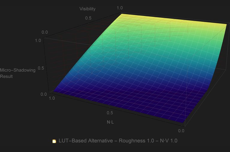
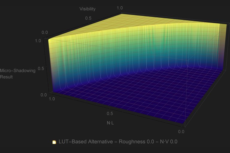
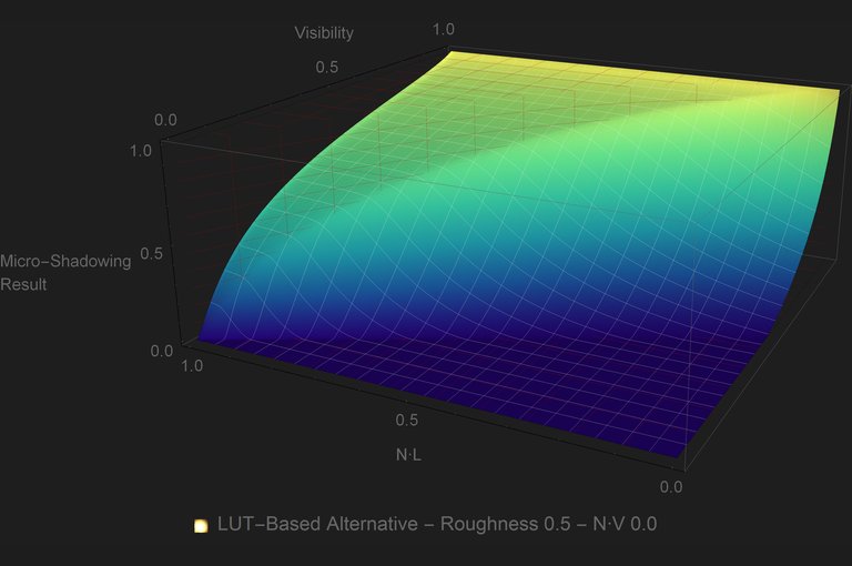
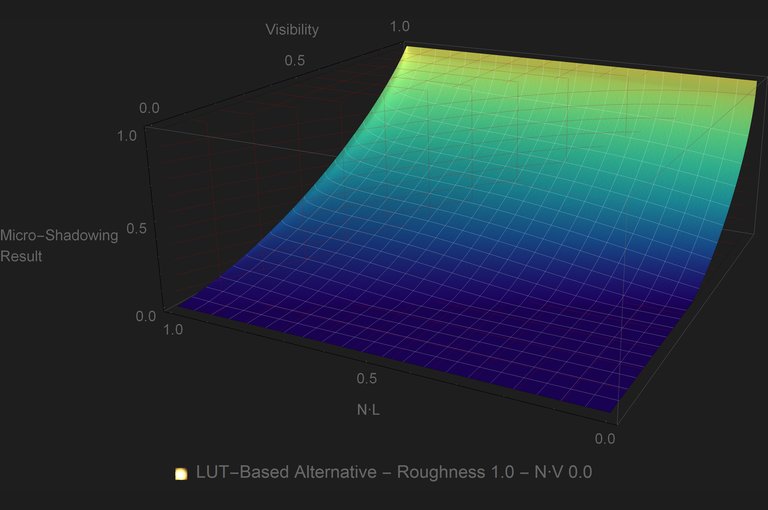
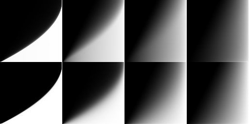
Let’s look at some plots of the micro-shadowing in a similar fashion as in part 1 but with isotropic \({Roughness}\) (where isotropic GGX \({\alpha_{xy}={Roughness}^{2}}\)) and \({N\cdot V}\) as extra parameters:
 |
|---|
| Click to view plots. |
At \({Roughness=0.0}\) the function follows the reference function, both ends of the \({Visibility}\) range returns what’s expected, and there is a change of the micro-shadowing based on \({\left\langle \omega_{g}\cdot \omega_{i} \right\rangle}\) aka \({N\cdot V}\). What’s also visible comparing the two rows of plots is that, if necessary and at a quality cost, the micro-shadowing can be simplified assuming that \({\left\langle \omega_{g}\cdot \omega_{i} \right\rangle = 1}\). But enough with the math and plots, lets look at the results on the comparison scene.
 |
|---|
| Visual results. |
The results look good, but it doesn’t show how micro-shadowing changes based on \({Roughness}\). Let’s look at a test case.
 |
|---|
| Damaged plaster texture set on a flat plane with high roughness on the left half, and low roughness on the right half. Notice how the sharpness of the micro-shadowing changes with roughness. |
The results look good, but taking \(n\) number of samples, per light, per pixel can be slow. This is when it might make sense to trade off quality for performance by making a lookup table (LUT).
LUT-Based Approximation
The use of LUTs for this kind of approximations is quite common. Most PBR engines have at least the DFG LUT. But unlike the DFG LUT, the micro-shadowing LUT will have to be sampled per light, so it is important to avoid that where possible. Looking at the plots it is evident that for GGX there is a substantial area of the plot where the micro-shadowing result is \({0.0}\) no matter what the inputs are. That means that for that area of inputs we can skip the look up onto the LUT. If \({2{Visibility}+{\left\langle \omega_{g}\cdot \omega_{o} \right\rangle}\lt 1}\) then the micro-shadowing result is \({0.0}\).
While this micro-shadowing approach works just fine with anisotropic GGX, for some scenarios a reasonable compromise is to assume an isotropic GGX microsurface. That reduces the dimensions of the LUT and simplifies the implementation of \({GenericM_{m}(cos\,\theta,\omega_{m},\omega_{g},\omega_{o},\omega_{i})}\) to:
 1void MicroShadowingTermPZGenericVNDFBased_Isotropic(in float cosTheta, in float ggxAlpha, in float3 N, in float3 L, in float3 V, in float2 u1u2,
 2	out float outConeResult, out float outHemisphereResult, out float outSampleWeight)
 3{
 4	const float3 M = ImportanceSampleGGXVNDF_Isotropic(V, ggxAlpha, u1u2); // wm
 5
 6	const float NdotM = saturate(dot(N, M));
 7	const float MdotL = saturate(dot(M, L));
 8
 9	outSampleWeight = ImportanceSampleGGXVNDF_IsotropicWeight(V, L, M, ggxAlpha); // G2(wi,wo,wm)/G1(wi,wm)
10	outHemisphereResult = HeavisideFunction(NdotM) * HeavisideFunction(MdotL) * outSampleWeight;
11	outConeResult = HeavisideFunction(NdotM - cosTheta) * HeavisideFunction(MdotL - cosTheta) * outSampleWeight;
12}
Another reasonable compromise is to clamp \(Roughness\) to a non-zero value. Limiting the LUT \(Roughness\) to \({[0.1, 1.0]}\) allows for a bit smoother transition in the micro-shadow at low \(Roughness\), while at the same time lowering the number of \(Roughness\) slices required.
Based on those compromises, a LUT can be created that is parametrized by \({Visibility}\), \({Roughness}\), \({N\cdot L}\), and \({N\cdot V}\). There are many options for how to store and sample that in a LUT, but as a simple naive example, a single RGBA_UNORM 3D texture can be used where \({x = Visibility}\) increasing from left to right, \({y = N\cdot L}\) increasing from top to bottom, and \({z = N\cdot V}\) increasing in depth. On each channel \(Roughness\) can stored where \({r = 0.1}\), \({g = 0.4}\), \({b = 0.7}\), and \({a = 1.0}\).
 |
|---|
| Slices of the 3D LUT with increasing \(Roughness\) left to right and increasing \({N\cdot V}\) top to bottom. The 2D LUT is just the second slice that corresponds to \({N\cdot V=1}\). |
The 2D LUT provides an even more compact representation but at the quality cost of assuming \({N\cdot V=1}\). While the LUT may not reflect as big of a change in the values, the impact can be quite substantial for specular as seen below. With that said, it may still be a reasonable compromise depending on the resource constraints.
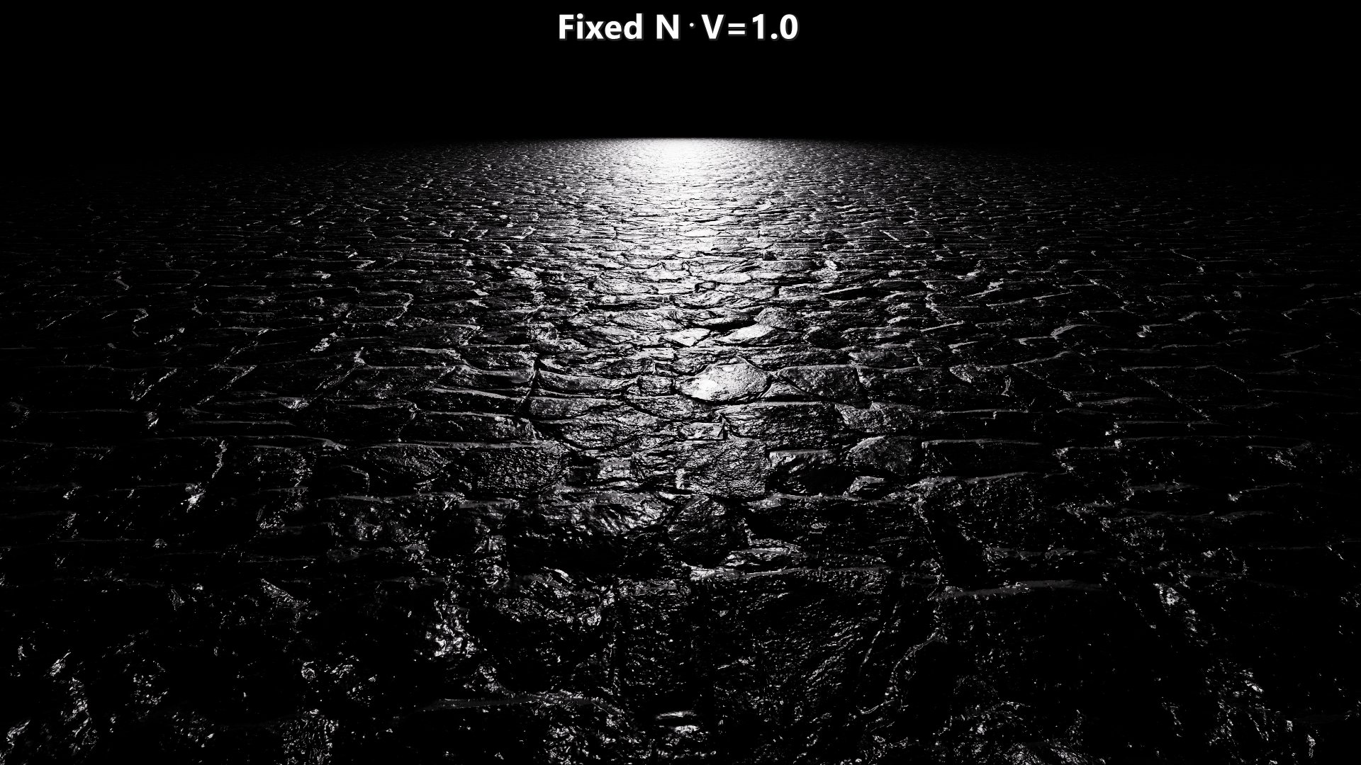
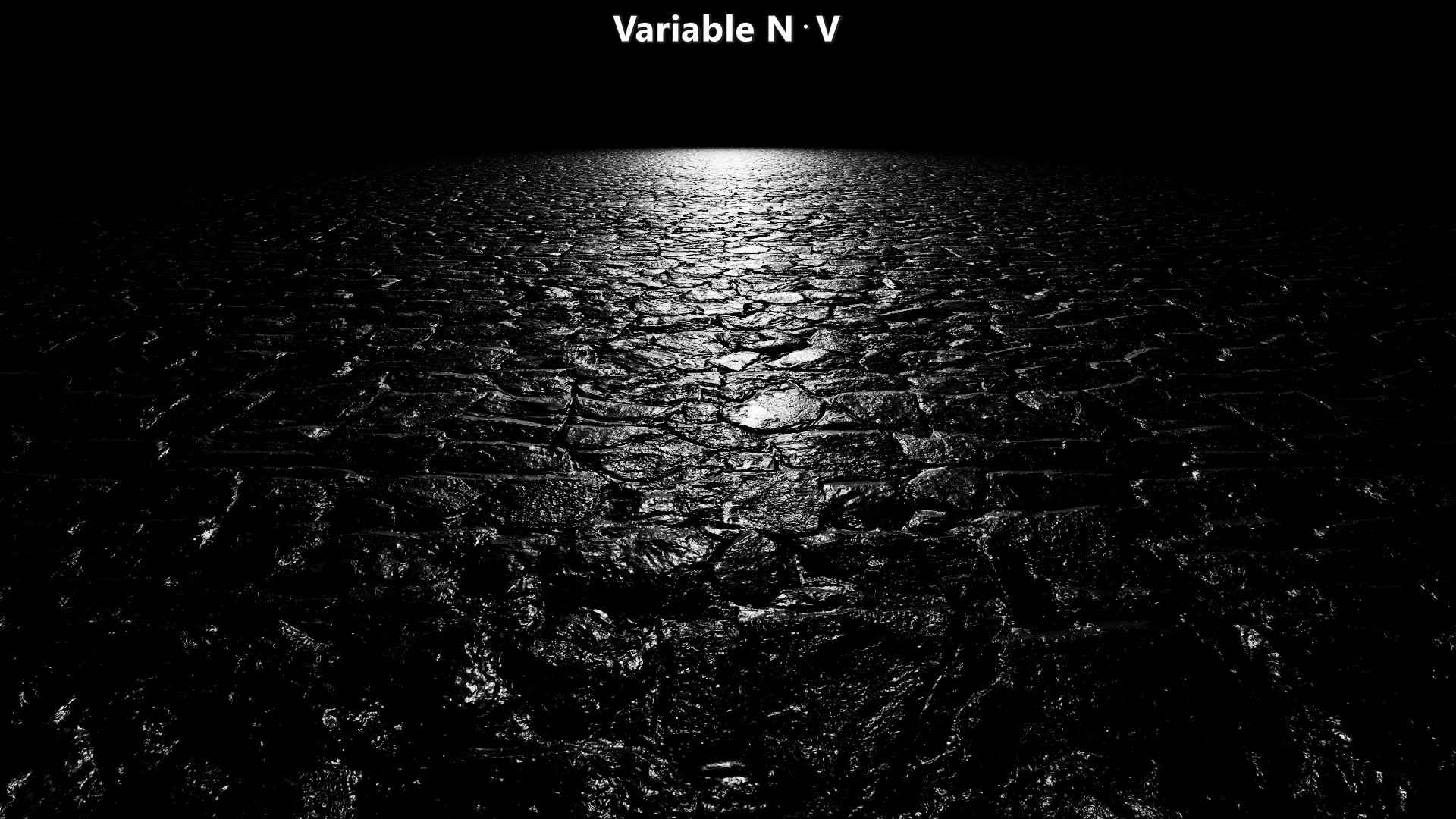 |
|---|
| Quality impact on micro-shadowing the specular component assuming \({N\cdot V=1}\) versus a variable \({N\cdot V}\). |
Next Time
In this post I have been referring to this approach as Generic VNDF-Based Micro-Shadowing. The reason for using “Generic” as a term is that the approach as shown here isn’t aware of the micro-BRDF of the microfacets. As is, this approach assumes that if a microfacet is visible through the visibility cone, then both the specular reflection of the light on the microfacet and the diffuse reflected directions on the microfacet are also visible through the visibility cone. That creates a fair amount of under occlusion, so improving that will be the focus for a future post. The other issue for a future post is the handling of area lights that are not implemented using the “representative point” approach.
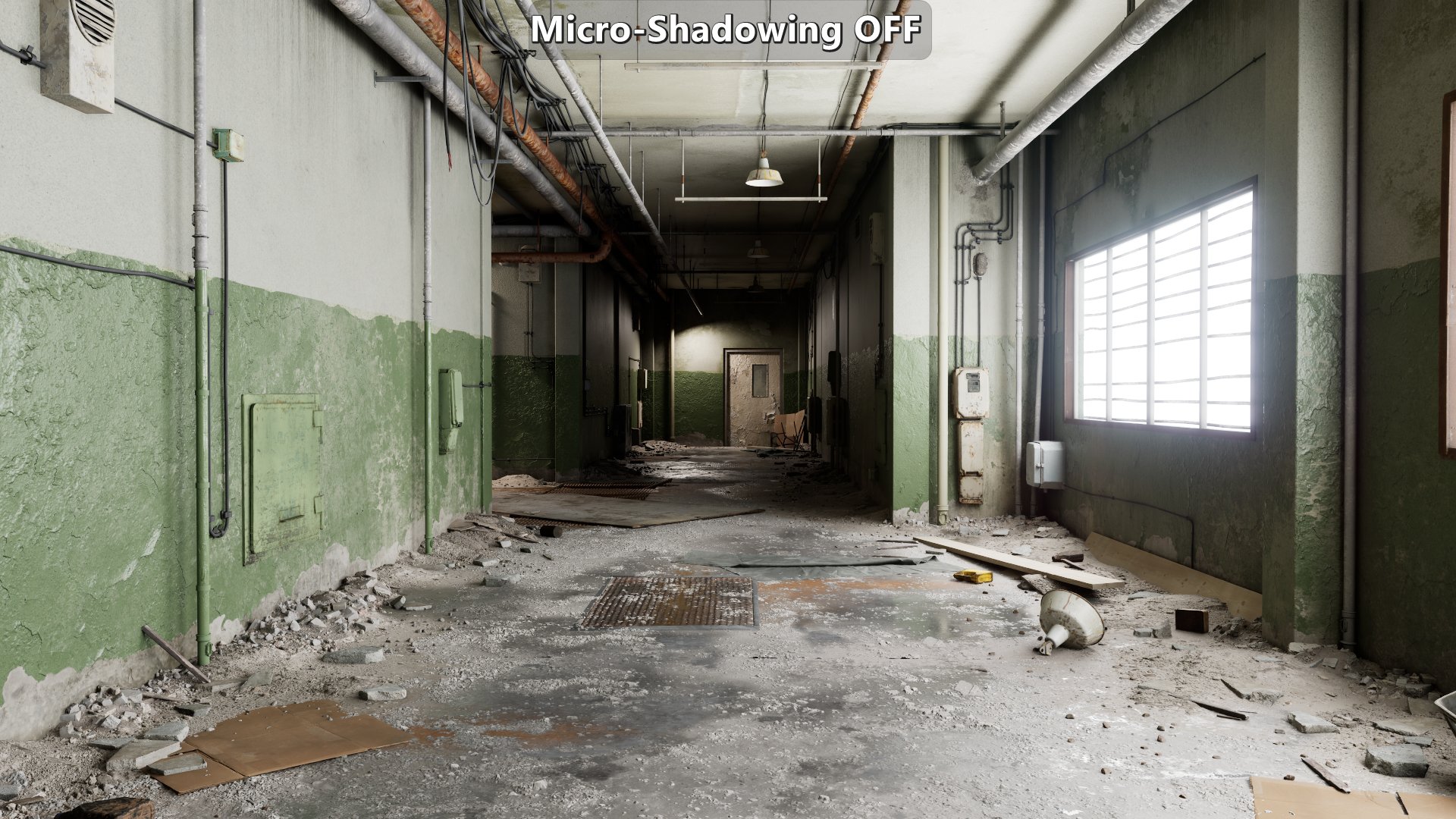
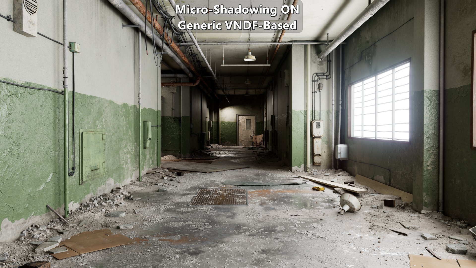
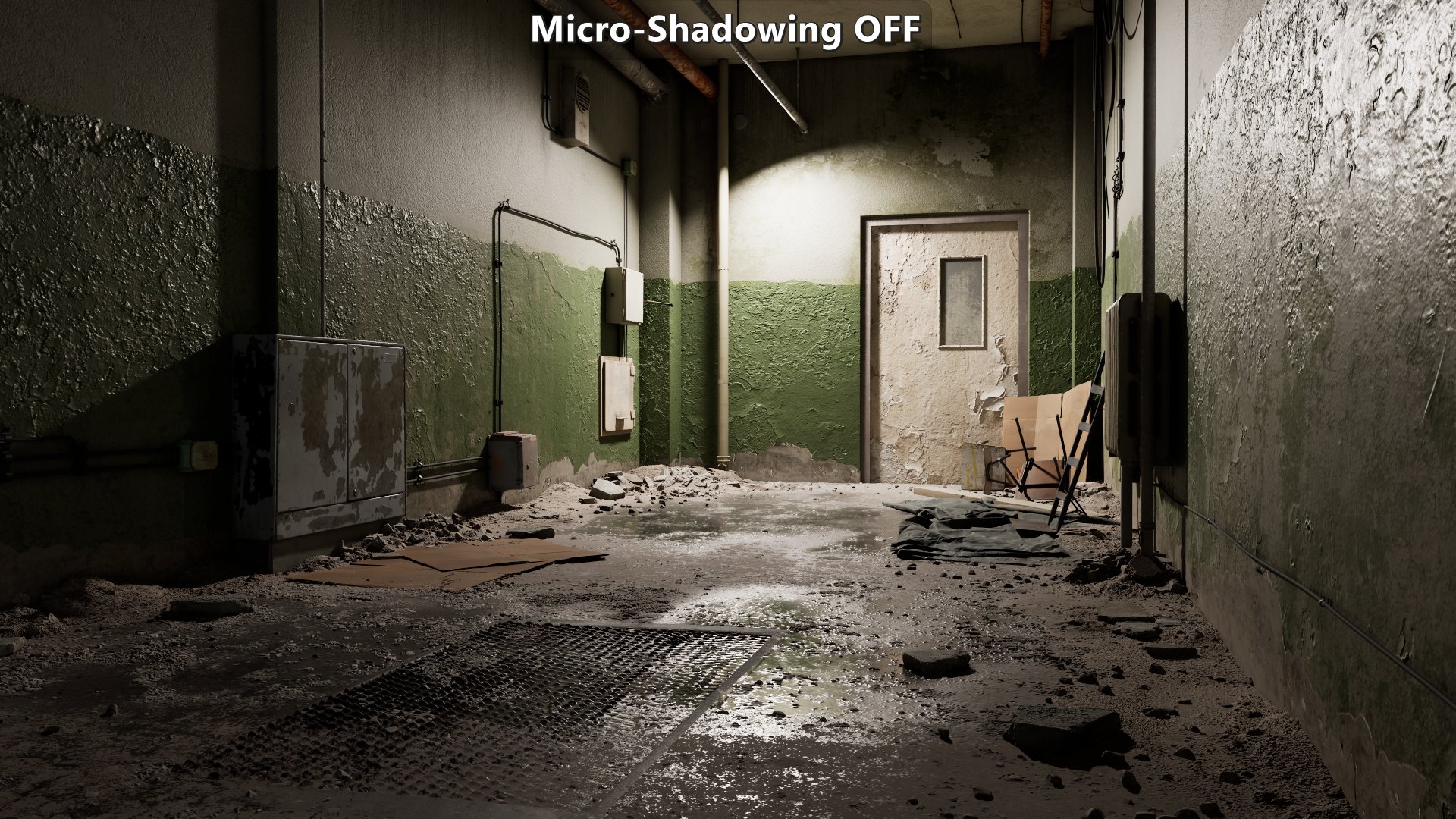
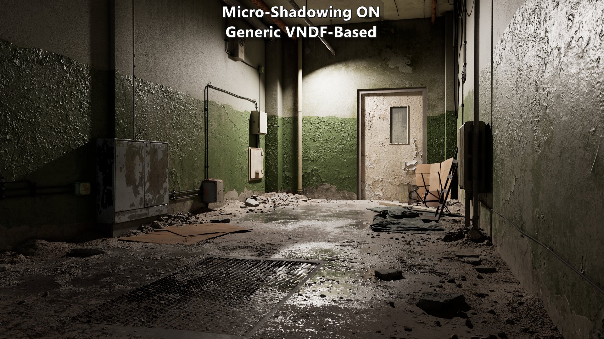
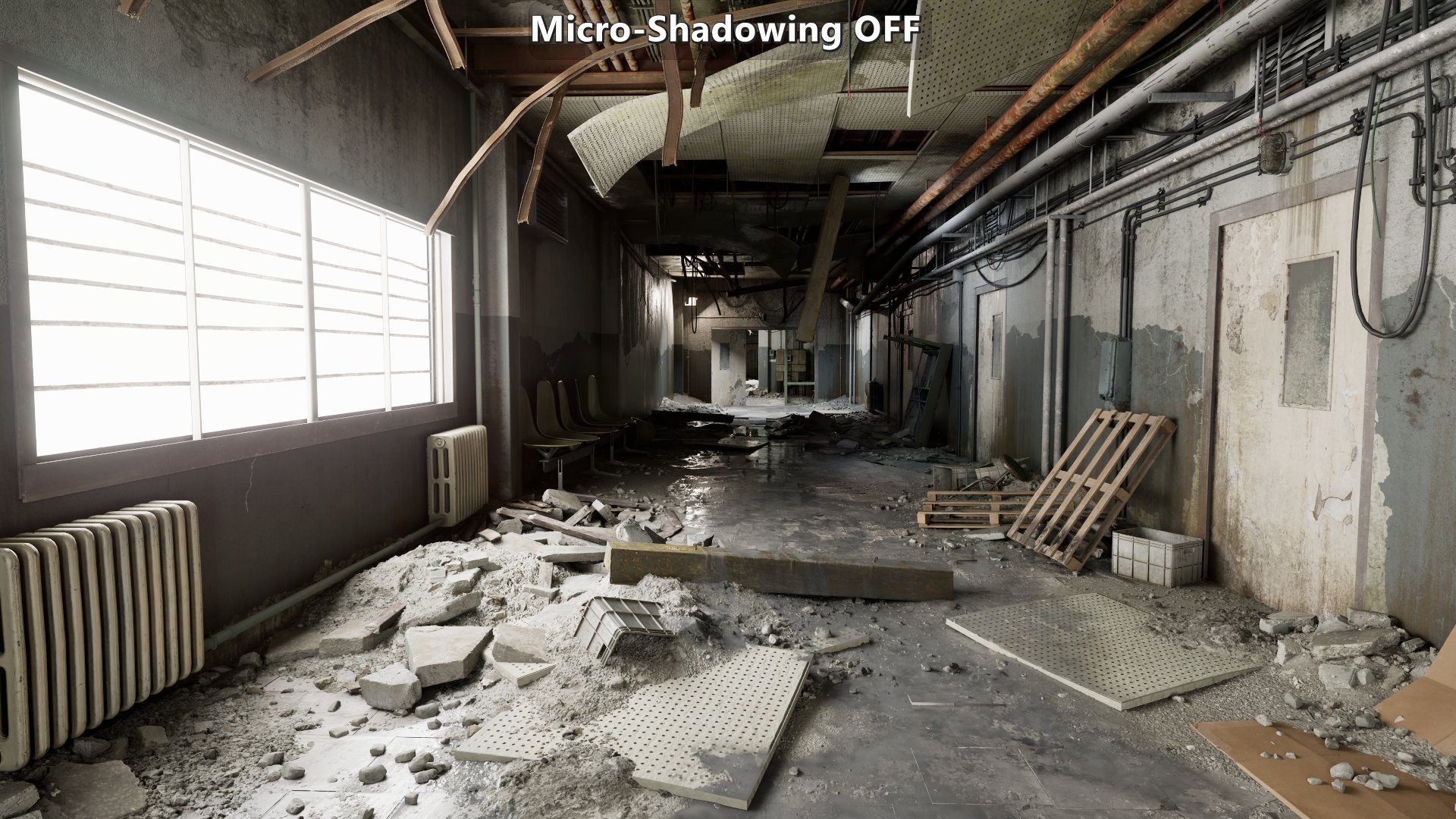
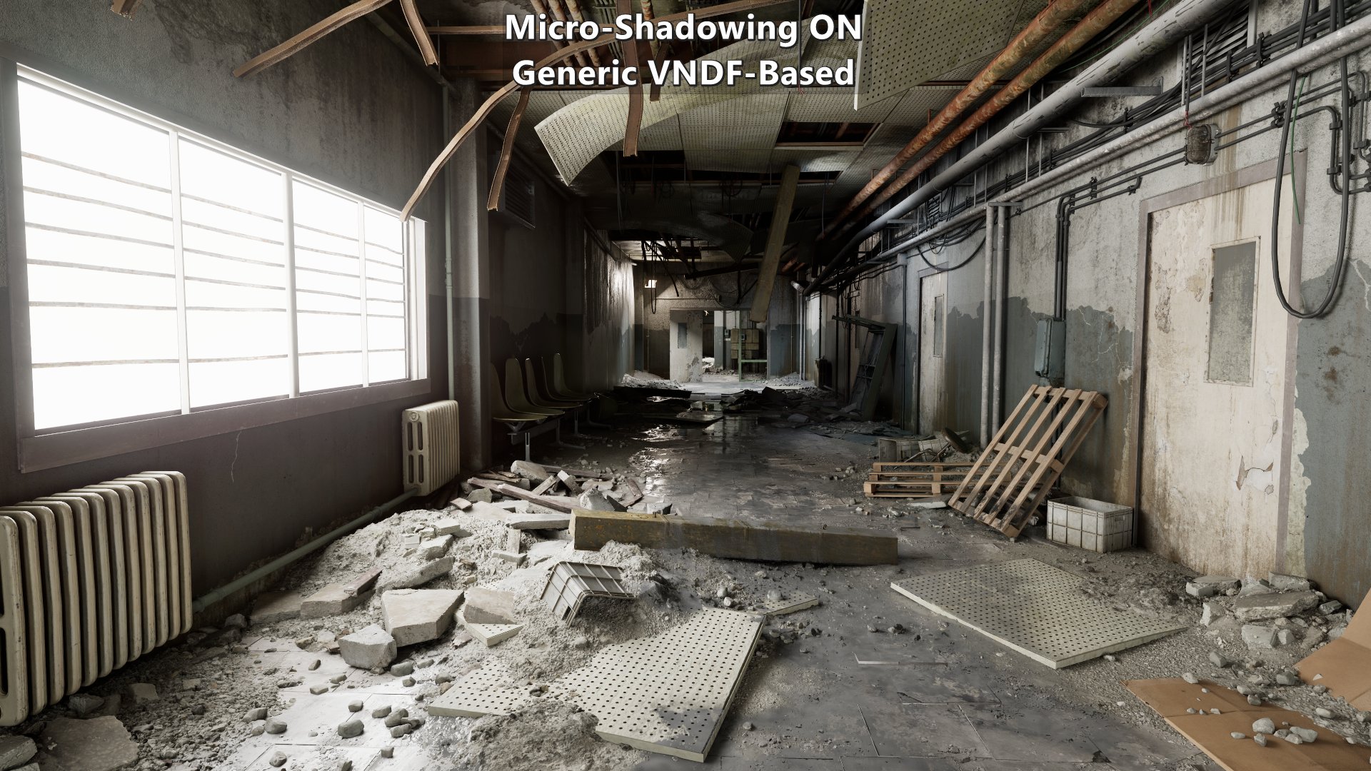
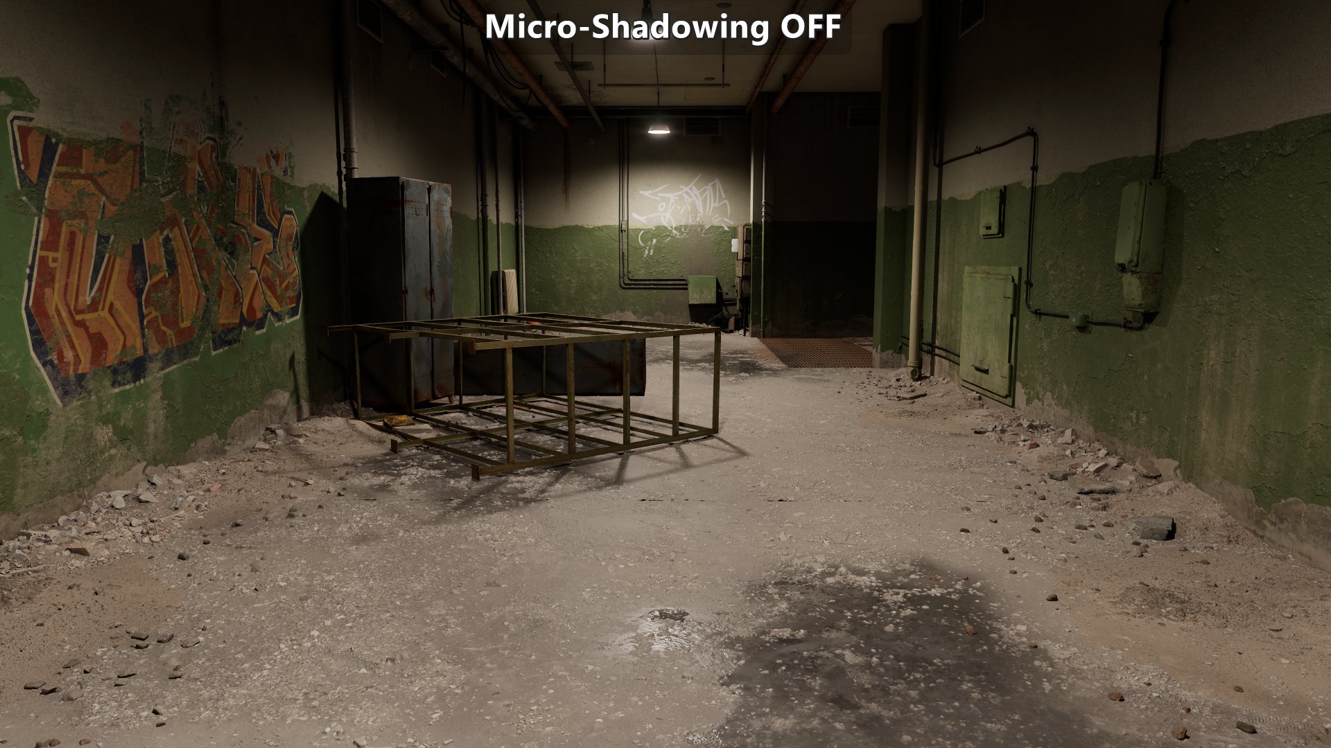
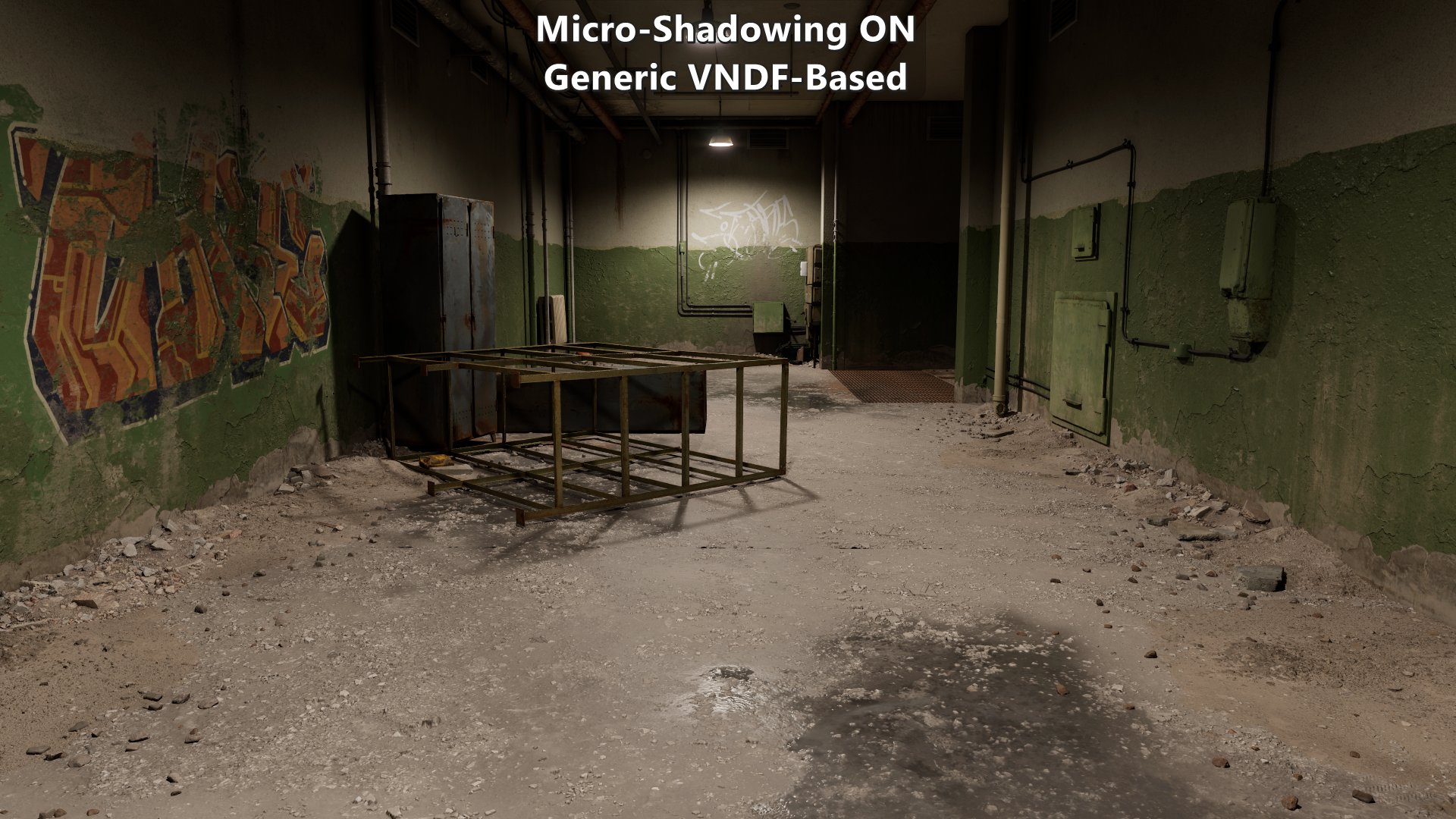
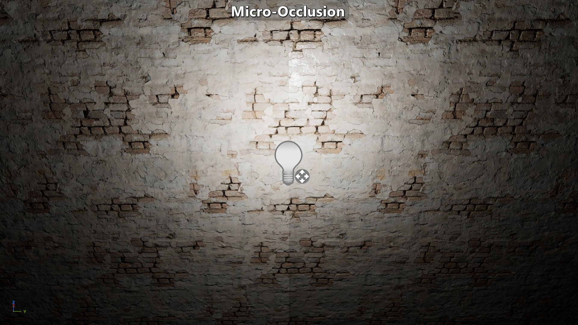
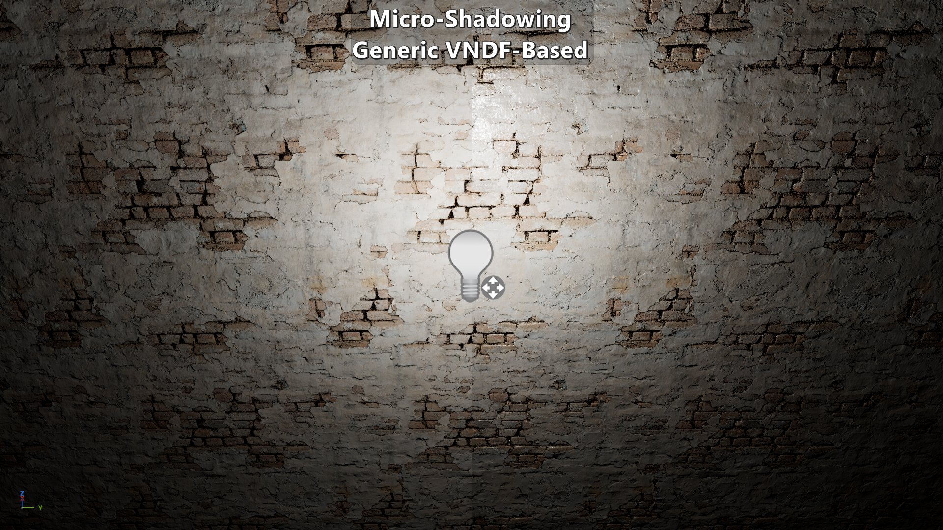
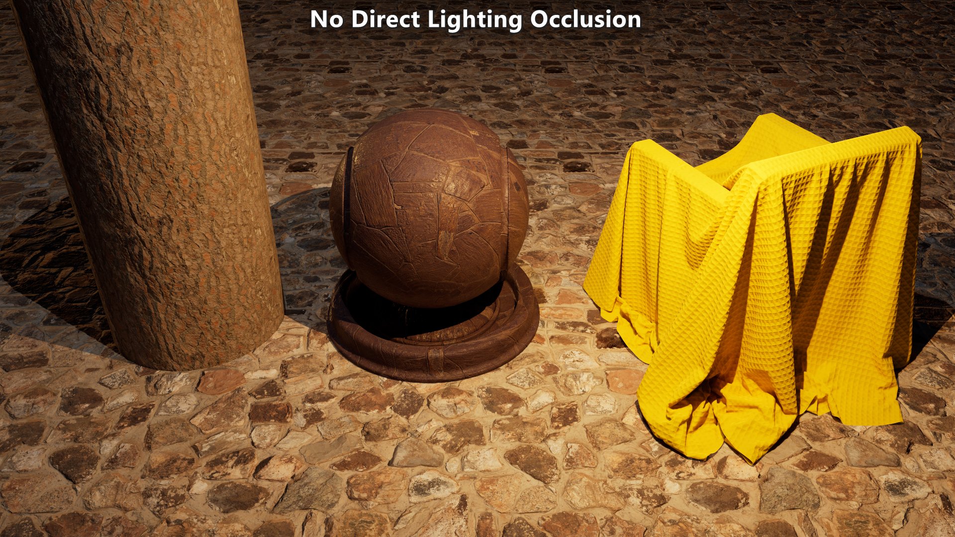
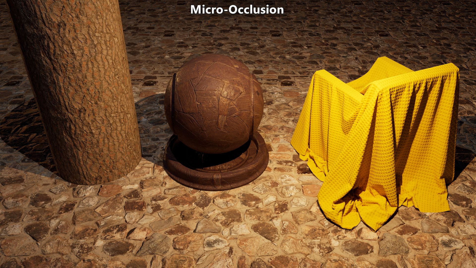
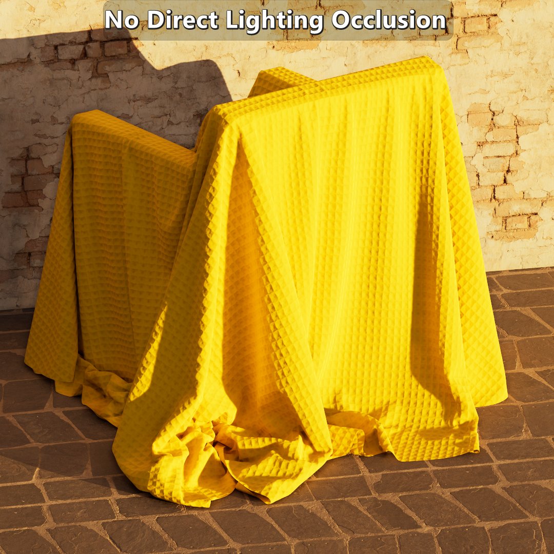
Results
The results shown here are only meant to represent the visual impact of the feature under the same conditions, and using the 3D LUT approximation. There isn’t any tuning of the materials based on distance, view direction, et cetera. None of the content shown here was created with micro-shadowing in mind which means that qualitative comparisons are not as relevant. With that said, they still reflect the differences among the approaches.
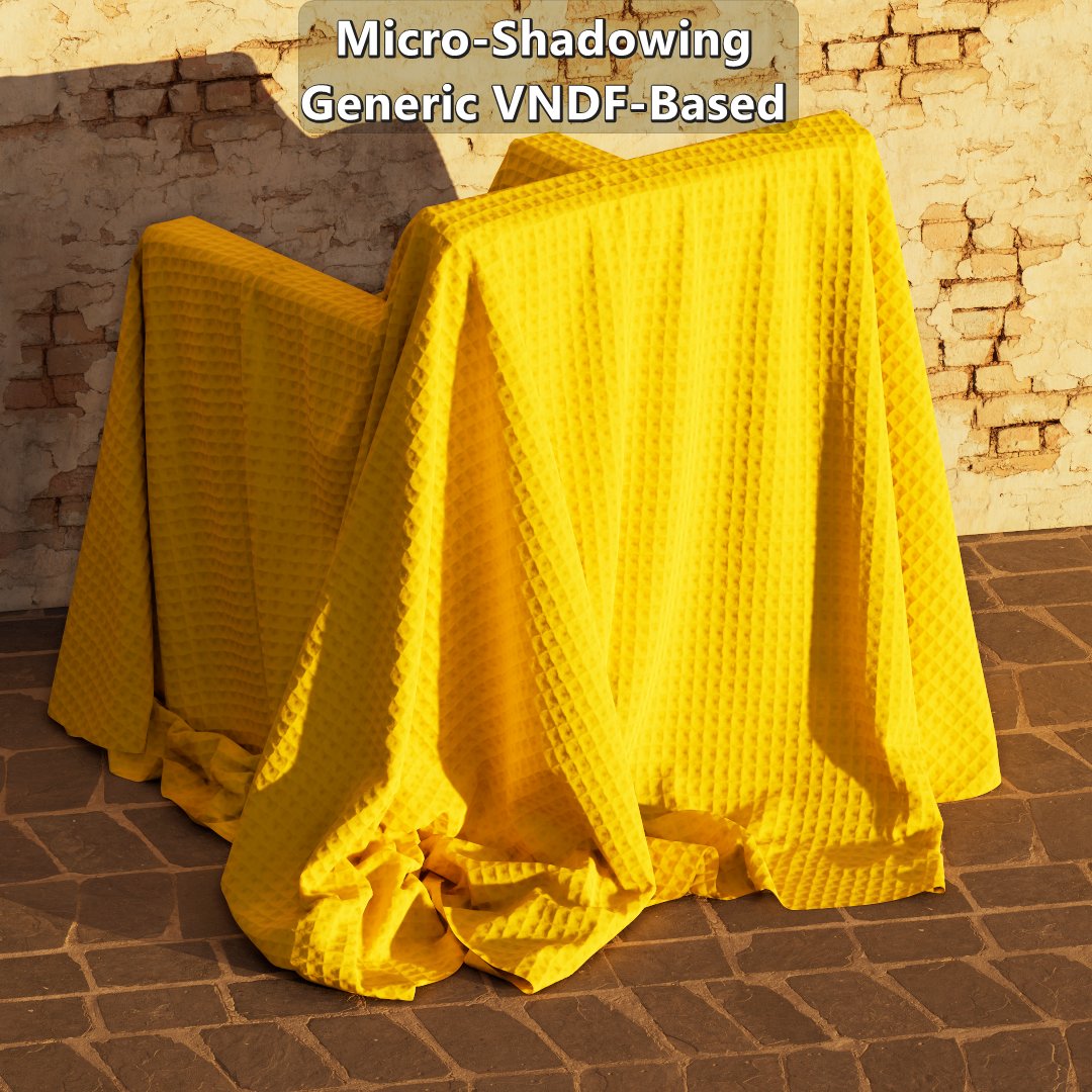
Multiple Materials
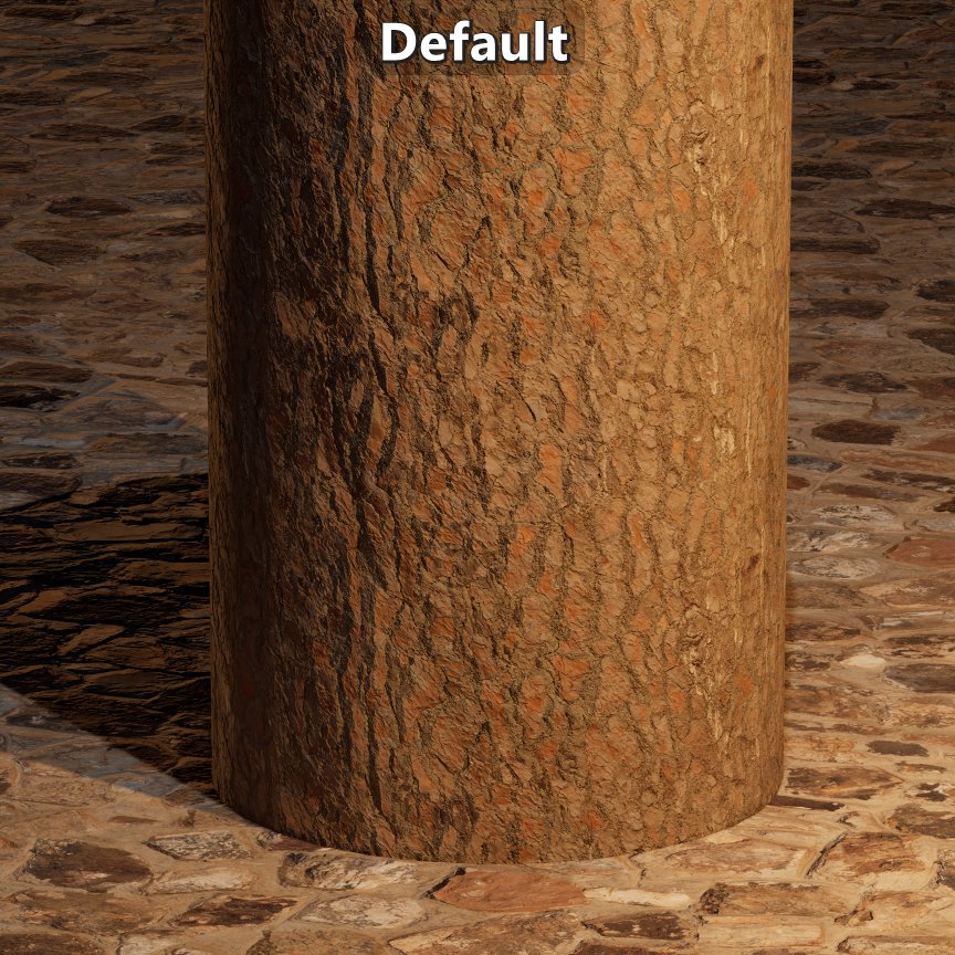
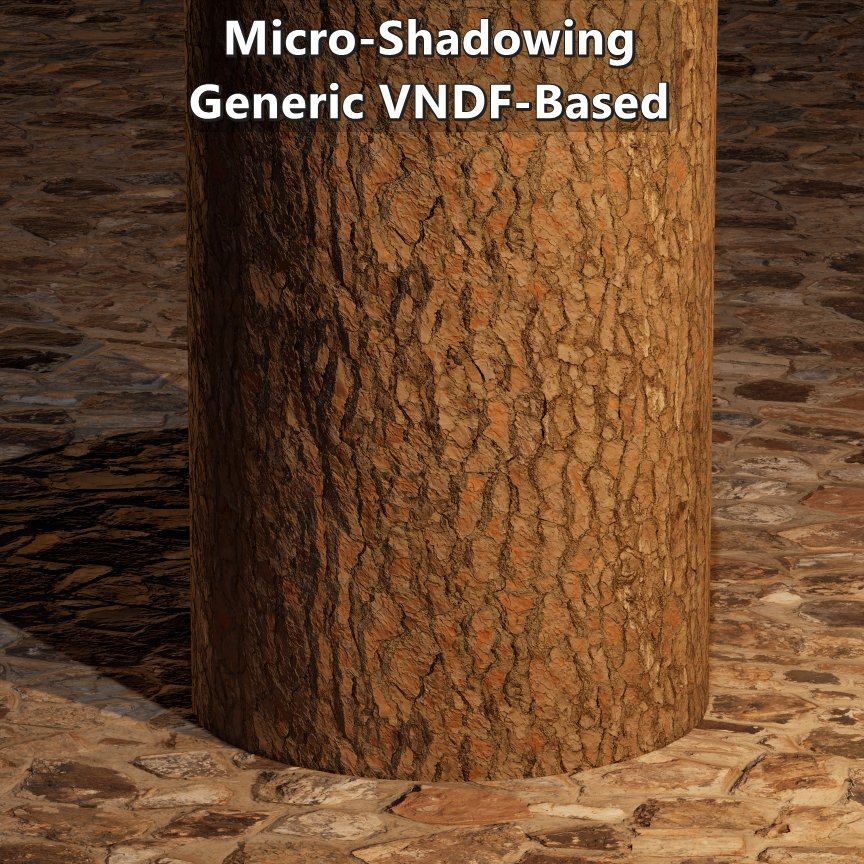
Same micro-occlusion data in all shots. Notice how micro-shadowing doesn’t double up ambient occlusion and provides more shape depending on the light source.


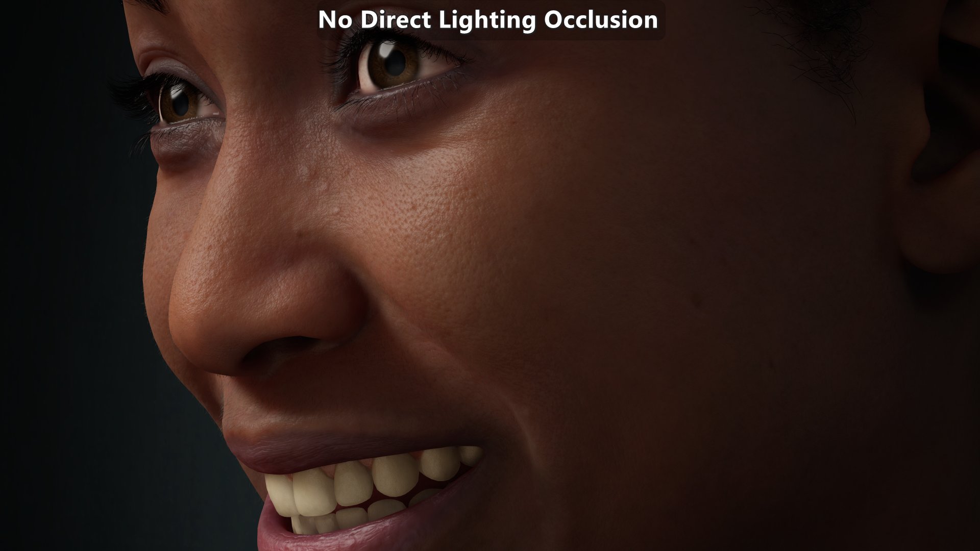
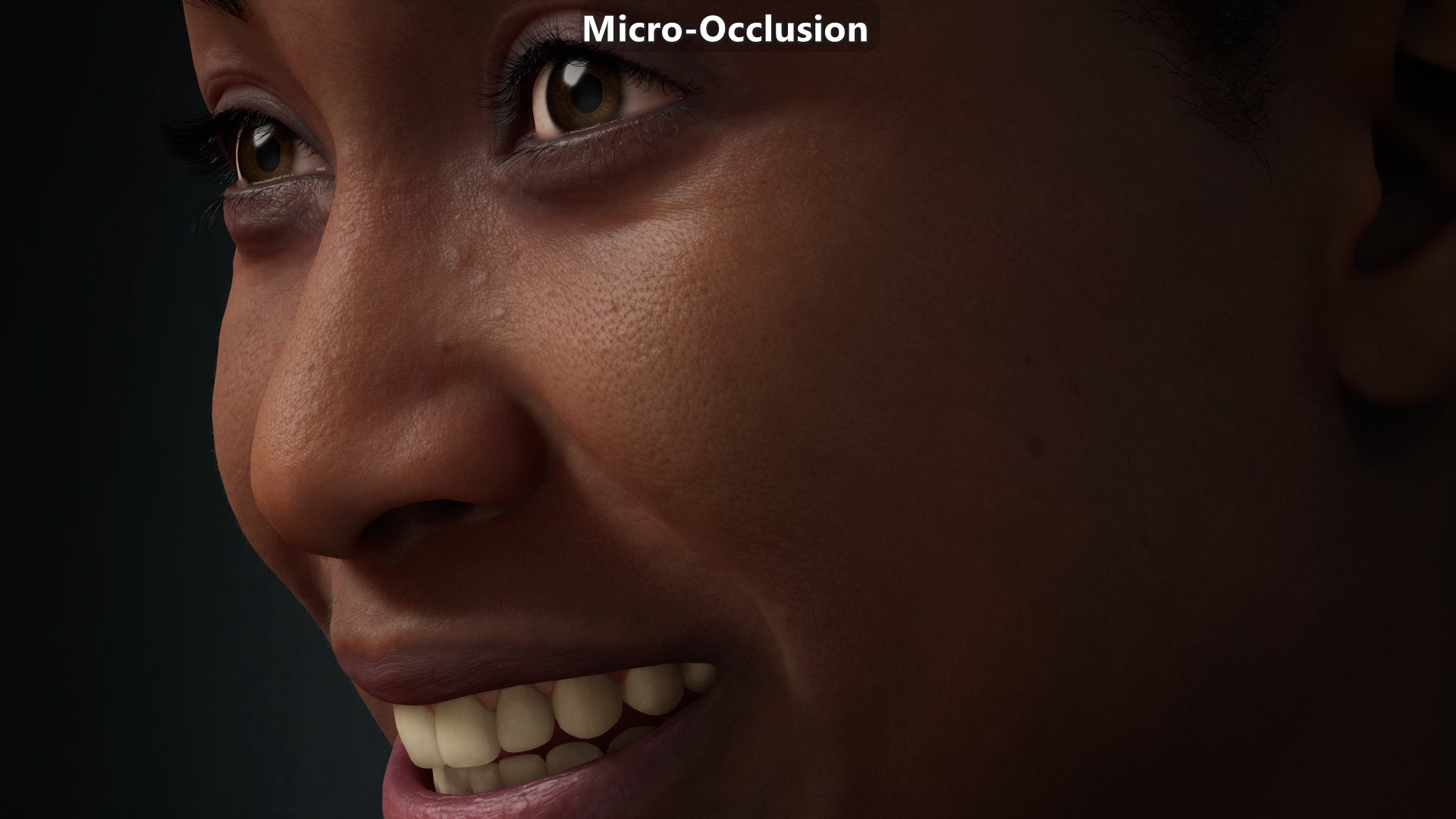
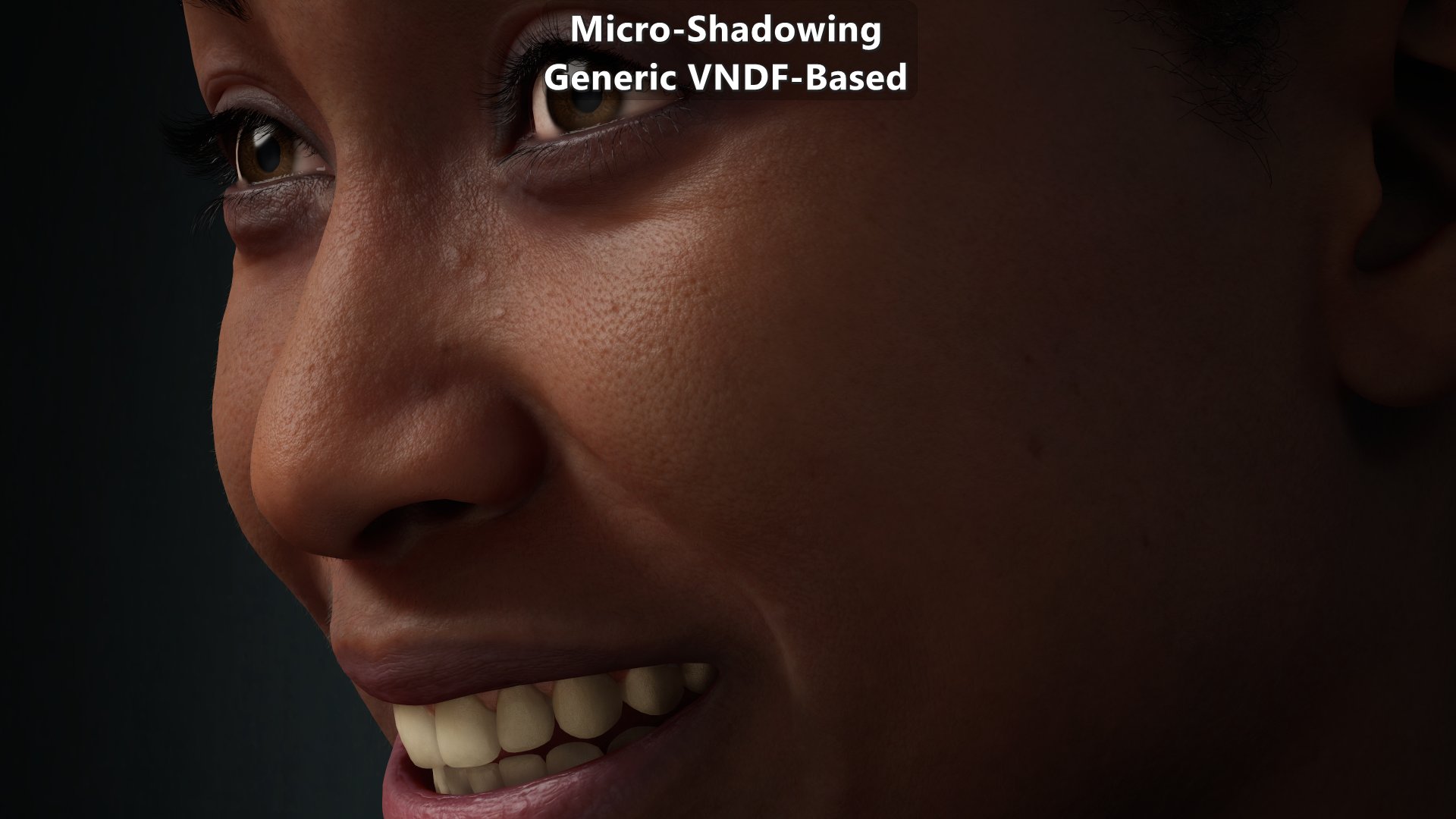
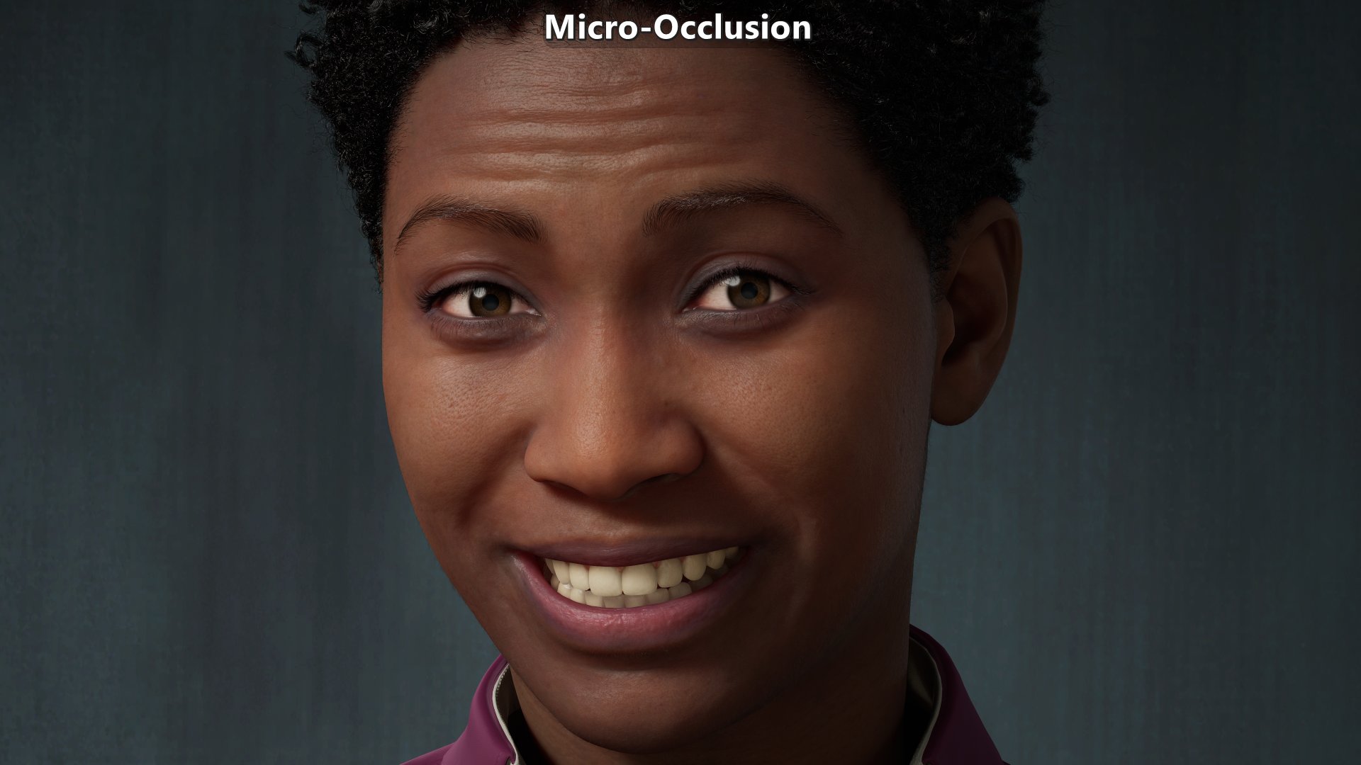
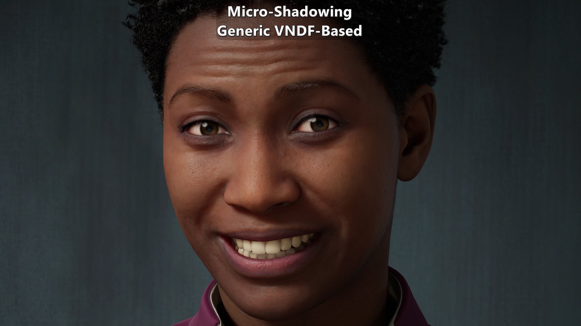
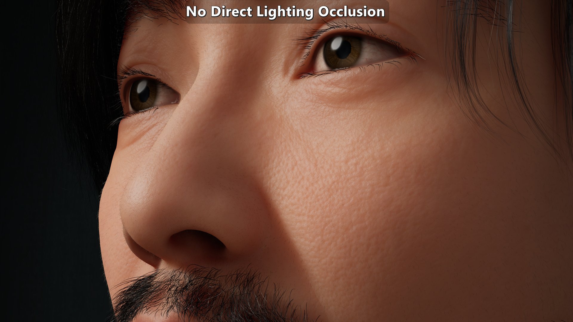
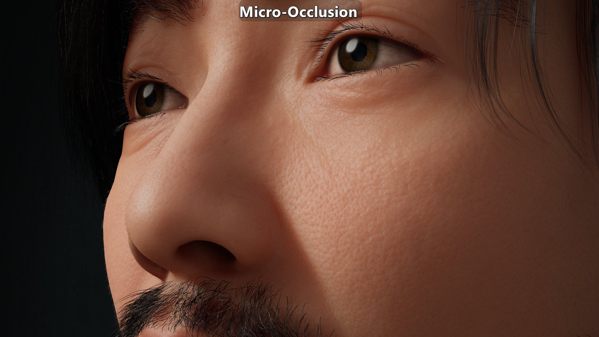
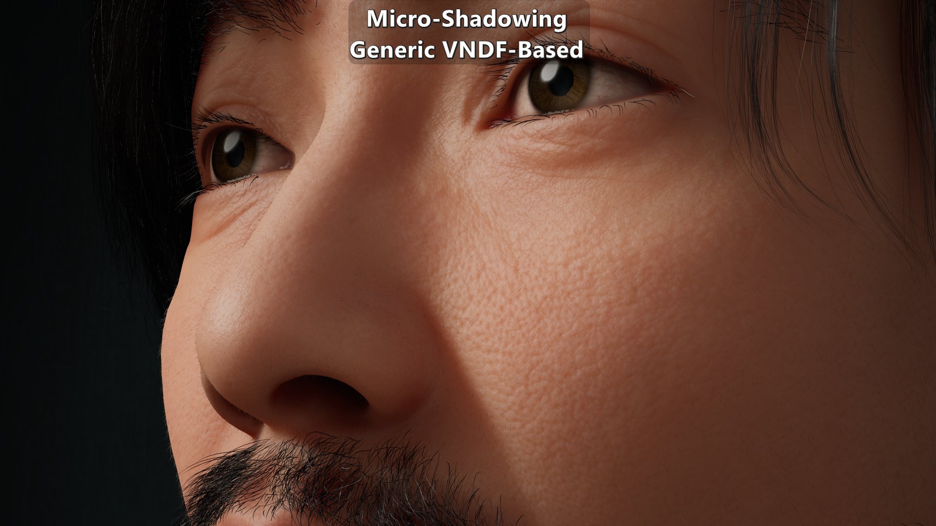
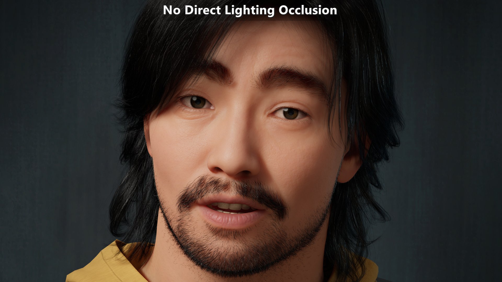
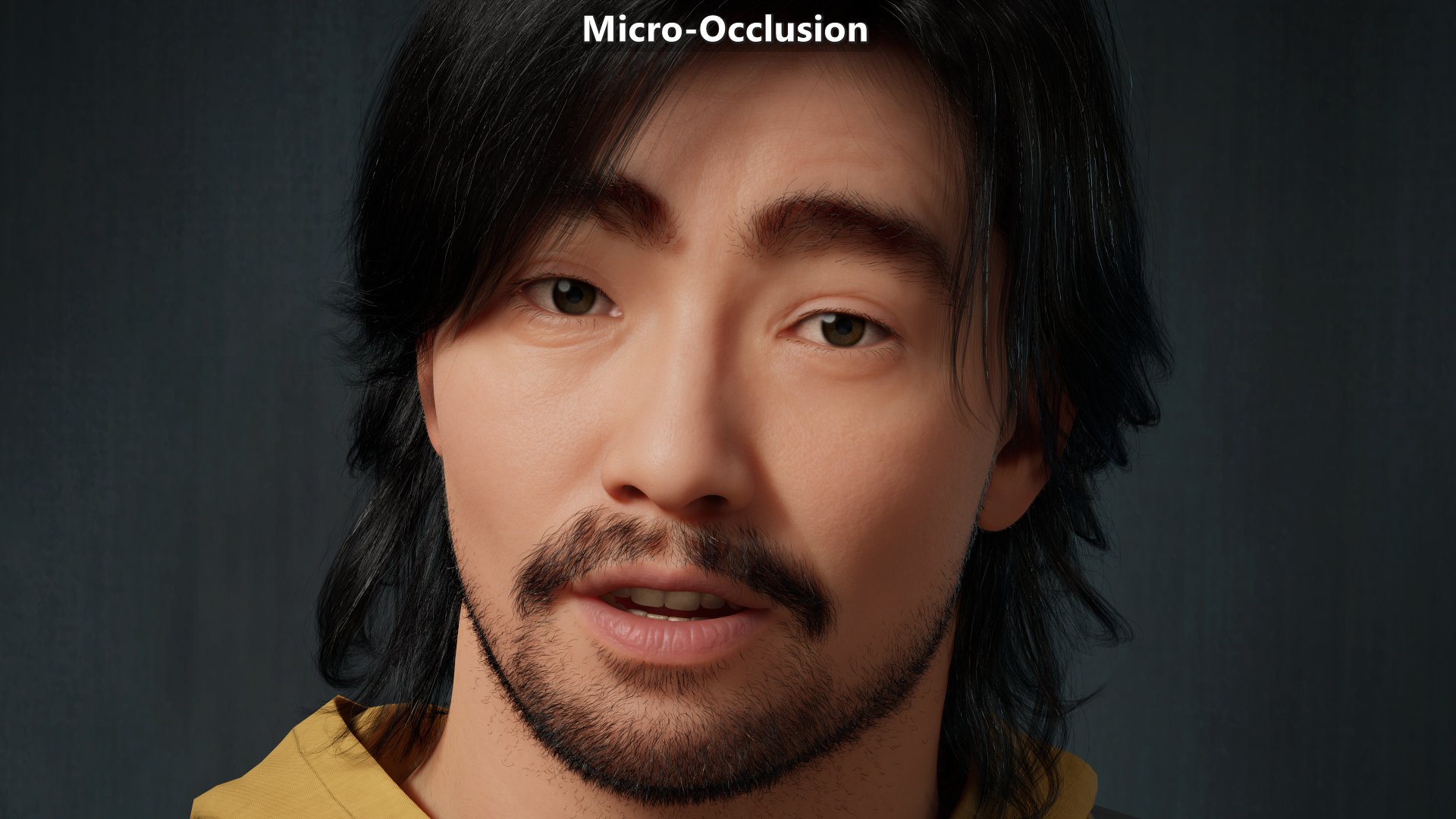
MetaHuman
Modified version of a MetaHuman sample. Animated albedo disabled, shaders and subsurface profiles modified to make them move physically based. Micro-occlusion data is the same on close ups and further away. The key light is on the right from the character’s point of view which explains why the left side of the character from their point of view shows more micro-shadowing
Ada

Taro
Derelict Corridor
Modified version of a Quixel Megascans sample. Most of the changes were done to approximate micro-occlusion data from regular ambient occlusion data that came with the content.